RSF spring-block simulations

In this tutorial, we’ll run a series of spring-block (1D fault) simulations with the classical rate-and-state friction framework. The corresponding Jupyter Notebook file is found in examples/notebooks/CNS_spring-block.ipynb. We start by importing the necessary libraries:

# Make plots interactive in the notebook
%matplotlib notebook

import matplotlib.pyplot as plt
import numpy as np

import os
import sys

# Add QDYN source directory to PATH
# Go up in the directory tree
upup = [os.pardir]*2
qdyn_dir = os.path.join(*upup)
# Get QDYN src directory
src_dir = os.path.abspath(
    os.path.join(
        os.path.join(os.path.abspath(""), qdyn_dir), "src")
)
# Append src directory to Python path
sys.path.append(src_dir)

# Import QDYN wrapper
from pyqdyn import qdyn

The simulation parameters are accessible after instantiation of the QDYN class as a Python dictionary object. We first define a number of global simulation parameters:

# Instantiate the QDYN class object
p = qdyn()

# Get the settings dict
set_dict = p.set_dict

# Global simulation parameters
set_dict["MESHDIM"] = 0        # Simulation dimensionality (spring-block)
set_dict["TMAX"] = 300         # Maximum simulation time [s]
set_dict["NTOUT"] = 100        # Save output every N steps
set_dict["V_PL"] = 1e-5        # Load-point velocity [m/s]
set_dict["MU"] = 2e9           # Shear modulus [Pa]
set_dict["SIGMA"] = 5e6        # Effective normal stress [Pa]
set_dict["ACC"] = 1e-7         # Solver accuracy
set_dict["SOLVER"] = 2         # Solver type (Runge-Kutta)

# To switch to rate-and-state friction ("RSF")
set_dict["FRICTION_MODEL"] = "RSF"

We then overwrite the default values of specific rheological parameters:

set_dict["SET_DICT_RSF"]["RNS_LAW"] = 0               # Classical rate-and-state
set_dict["SET_DICT_RSF"]["THETA_LAW"] = 1             # Ageing law
set_dict["SET_DICT_RSF"]["A"] = 0.01                  # Direct effect parameter [-]
set_dict["SET_DICT_RSF"]["B"] = 0.015                 # Evolution effect parameters [-]
set_dict["SET_DICT_RSF"]["DC"] = 1e-5                 # Characteristic slip distance [m]
set_dict["SET_DICT_RSF"]["V_SS"] = set_dict["V_PL"]   # Reference velocity [m/s]

# Initial slip velocity [m/s]
set_dict["SET_DICT_RSF"]["V_0"] = 1.01 * set_dict["V_PL"]
# Initial state [s]
set_dict["SET_DICT_RSF"]["TH_0"] = set_dict["SET_DICT_RSF"]["DC"] / set_dict["V_PL"]

Lastly, we pass the settings to the QDYN wrapper, generate the mesh (only 1 element) and write the qdyn.in input file:

p.settings(set_dict)
p.render_mesh()
p.write_input()

The p.write() command writes a qdyn.in file to the current working directory, which is read by QDYN at the start of the simulation. To do this, call p.run(). Note that in this notebook, the screen output (stdout) is captured by the console, so you won’t see any output here.

p.run()

The simulation output is read and processed by the wrapper using:

p.read_output()

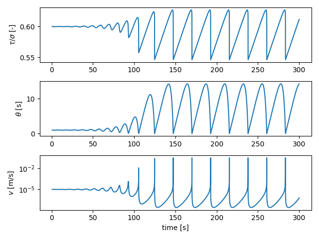
The simulation time series output is then stored as a pandas DataFrame in p.ot. To see the behaviour of our spring-block fault, we can plot the time series of (normalised) shear stress, porosity, and slip velocity:

plt.figure()

# Normalised shear stress
plt.subplot(311)
plt.plot(p.ot[0]["t"], p.ot[0]["tau"] / set_dict["SIGMA"])
plt.ylabel(r"$\tau / \sigma$ [-]")

# State
plt.subplot(312)
plt.plot(p.ot[0]["t"], p.ot[0]["theta"])
plt.ylabel(r"$\theta$ [s]")

# Velocity
plt.subplot(313)
plt.plot(p.ot[0]["t"], p.ot[0]["v"])
plt.yscale("log")
plt.ylabel(r"$v$ [m/s]")
plt.xlabel("time [s]")

plt.tight_layout()
plt.show()

Stick-slip