CNS spring-block simulations

In this tutorial, we’ll run a series of spring-block (1D fault) simulations with the Chen-Niemeijer-Spiers (CNS) microphysical model. The corresponding Jupyter Notebook file is found in examples/notebooks/CNS_spring-block.ipynb. We start by importing the necessary libraries:

# Make plots interactive in the notebook
%matplotlib notebook

import matplotlib.pyplot as plt
import numpy as np

import os
import sys

# Add QDYN source directory to PATH
# Go up in the directory tree
upup = [os.pardir]*2
qdyn_dir = os.path.join(*upup)
# Get QDYN src directory
src_dir = os.path.abspath(
    os.path.join(
        os.path.join(os.path.abspath(""), qdyn_dir), "src")
)
# Append src directory to Python path
sys.path.append(src_dir)

# Import QDYN wrapper
from pyqdyn import qdyn

The simulation parameters are accessible after instantiation of the QDYN class as a Python dictionary object. We first define a number of global simulation parameters:

# Instantiate the QDYN class object
p = qdyn()

# Get the settings dict
set_dict = p.set_dict

# Global simulation parameters
set_dict["MESHDIM"] = 0        # Simulation dimensionality (spring-block)
set_dict["TMAX"] = 200         # Maximum simulation time [s]
set_dict["NTOUT"] = 100        # Save output every N steps
set_dict["V_PL"] = 1e-5        # Load-point velocity [m/s]
set_dict["MU"] = 2e9           # Shear modulus [Pa]
set_dict["VS"] = 0             # Turn of radiation damping
set_dict["SIGMA"] = 5e6        # Effective normal stress [Pa]
set_dict["ACC"] = 1e-7         # Solver accuracy
set_dict["SOLVER"] = 2         # Solver type (Runge-Kutta)

# To switch from rate-and-state friction ("RSF"; default) to the CNS model,
# we set the "FRICTION_MODEL" to "CNS"
set_dict["FRICTION_MODEL"] = "CNS"

We then overwrite the default values of specific rheological parameters:

set_dict["SET_DICT_CNS"]["H"] = 0.5        # Dilatancy coefficient (higher = more dilatancy)
set_dict["SET_DICT_CNS"]["PHI_C"] = 0.3    # Critical state (maximum) porosity
set_dict["SET_DICT_CNS"]["A"] = [1e-10]    # Kinetic parameter of the creep mechanism
set_dict["SET_DICT_CNS"]["N"] = [1]        # Stress exponent of the creep mechanism

# Thickness of the (localised) gouge layer [m]
set_dict["SET_DICT_CNS"]["THICKNESS"] = 1e-4
# Initial shear stress [Pa]
set_dict["SET_DICT_CNS"]["TAU"] = 0.5 * set_dict["SIGMA"]
# Initial porosity [-]
set_dict["SET_DICT_CNS"]["PHI_INI"] = 0.25

Lastly, we pass the settings to the QDYN wrapper, generate the mesh (only 1 element) and write the qdyn.in input file:

p.settings(set_dict)
p.render_mesh()
p.write_input()

The p.write() command writes a qdyn.in file to the current working directory, which is read by QDYN at the start of the simulation. To do this, call p.run(). Note that in this notebook, the screen output (stdout) is captured by the console, so you won’t see any output here.

p.run()

The simulation output is read and processed by the wrapper using:

p.read_output()

The simulation time series output is then stored as a pandas DataFrame in p.ot. To see the behaviour of our spring-block fault, we can plot the time series of (normalised) shear stress, porosity, and slip velocity:

plt.figure()

# Normalised shear stress
plt.subplot(311)
plt.plot(p.ot[0]["t"], p.ot[0]["tau"] / set_dict["SIGMA"])
plt.ylabel(r"$\tau / \sigma$ [-]")

# Porosity
plt.subplot(312)
plt.plot(p.ot[0]["t"], 100 * p.ot[0]["theta"])
plt.ylabel(r"$\phi$ [%]")

# Velocity
plt.subplot(313)
plt.plot(p.ot[0]["t"], p.ot[0]["v"])
plt.yscale("log")
plt.ylabel(r"$v$ [m/s]")
plt.xlabel("time [s]")

plt.tight_layout()
plt.show()

Stick-slip

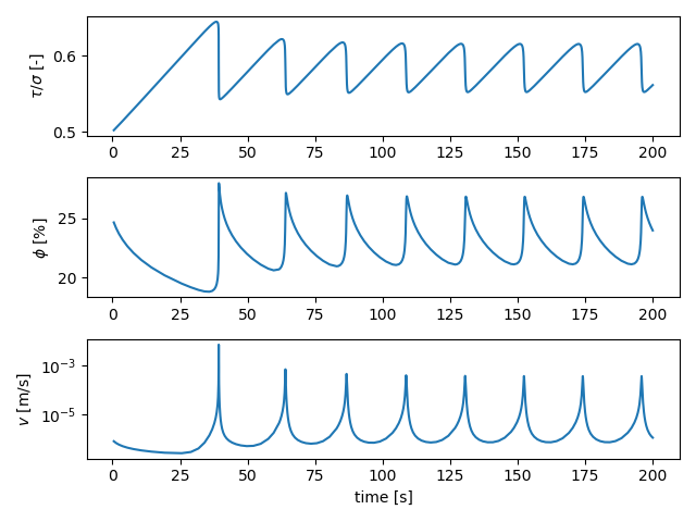
Note that the stick-slip cycles converge to a stable limit cycle, even in the absence of radiation damping. This is in contrast to classical rate-and-state friction, which does not exhibit stable limit cycles.

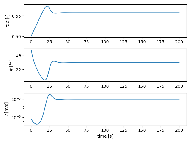
The stability of a fault governed by CNS rheology is very sensitive to the granular flow parameters, such as the dilatancy parameter $H$ (see van den Ende et al., 2018). By changing this value from 0.5 to 0.3, the fault stabilises at only deforms at steady-state:

set_dict["SET_DICT_CNS"]["H"] = 0.3        # Updated dilatancy coefficient

# Write settings, run simulation
p.settings(set_dict)
p.render_mesh()
p.write_input()
p.run()
p.read_output()

# Plot time series
plt.figure()
plt.subplot(311)
plt.plot(p.ot[0]["t"], p.ot[0]["tau"] / set_dict["SIGMA"])
plt.ylabel(r"$\tau / \sigma$ [-]")

plt.subplot(312)
plt.plot(p.ot[0]["t"], 100 * p.ot[0]["theta"])
plt.ylabel(r"$\phi$ [%]")

plt.subplot(313)
plt.plot(p.ot[0]["t"], p.ot[0]["v"])
plt.yscale("log")
plt.ylabel(r"$v$ [m/s]")
plt.xlabel("time [s]")

plt.tight_layout()
plt.show()

Stable